Excel is a great tool with a lot of flexibility and features to create and maintain records of information of any time. It also offers some fantastic visualization capabilities which is helpful when creating a trading journal.
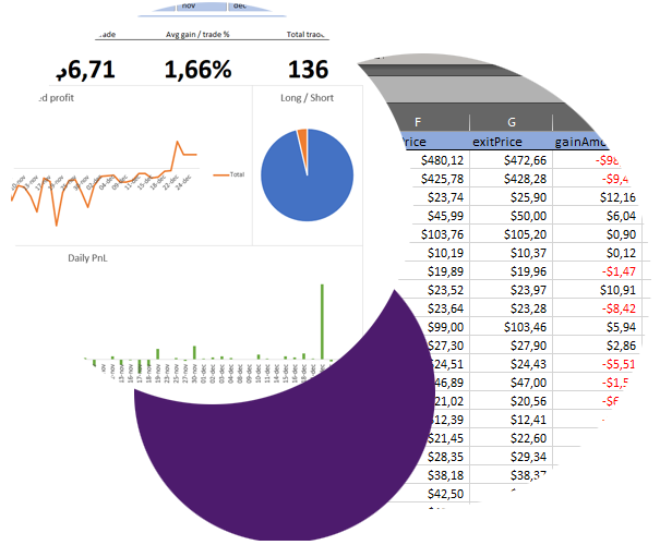
Google sheets is another alternative but to utilize all features and visualizations created in this tutorial I recommend using Microsoft Excel.
After completing this tutorial you will have
- A trading journal excel template
- A dynamic dashboard with time selection and charts to follow up your performance
It requires you to have basic knowledge of Excel but don´t worry, at the end of the tutorial you can download the completed excel trading journal template with some sample data.

What is a Trading Journal?
This tutorial assumes you have some basic understanding of what a trading journal is and how to use it. If you need to refresh your memory check the article What is a Trading Journal which goes through all the basics.
An alternative to use Excel for your trading journal is to use the kinfo trading journal to do journaling for you.
What should you put in your Excel trading journal
- Record trading information
- Follow up on results
- Identify improvements
- Correct your trading strategy
- Entry & Exit date
- Type (Long or Short)
- Symbol
- Entry & Exit Price
- PnL for the trade
- PnL in percent
- Win or Loss
In addition to the minimum requirements, most traders include one or more of the following data points:
- Timestamps
- Number of shares
- Fees
- Personal notes
- Tags to structure setups or strategies
- Number of trades
- Additional flags, for example if the trade was made following a strategy or deviating from it
- Asset class, Stock, Option, Future etc.
- Additional option information, Expiration, Put/Call, Spread information etc.
Getting started with Excel, adding columns
The first step is to startup excel and create a sheet for your trades.
You can use the first sheet name Sheet1 or rename it to Trades if you like.
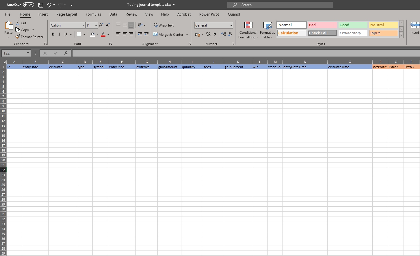
Add a column header for each data point you would like to track for each trade. In the example below we have used the minimum required data points and a few additional columns we want to track.
Adding data
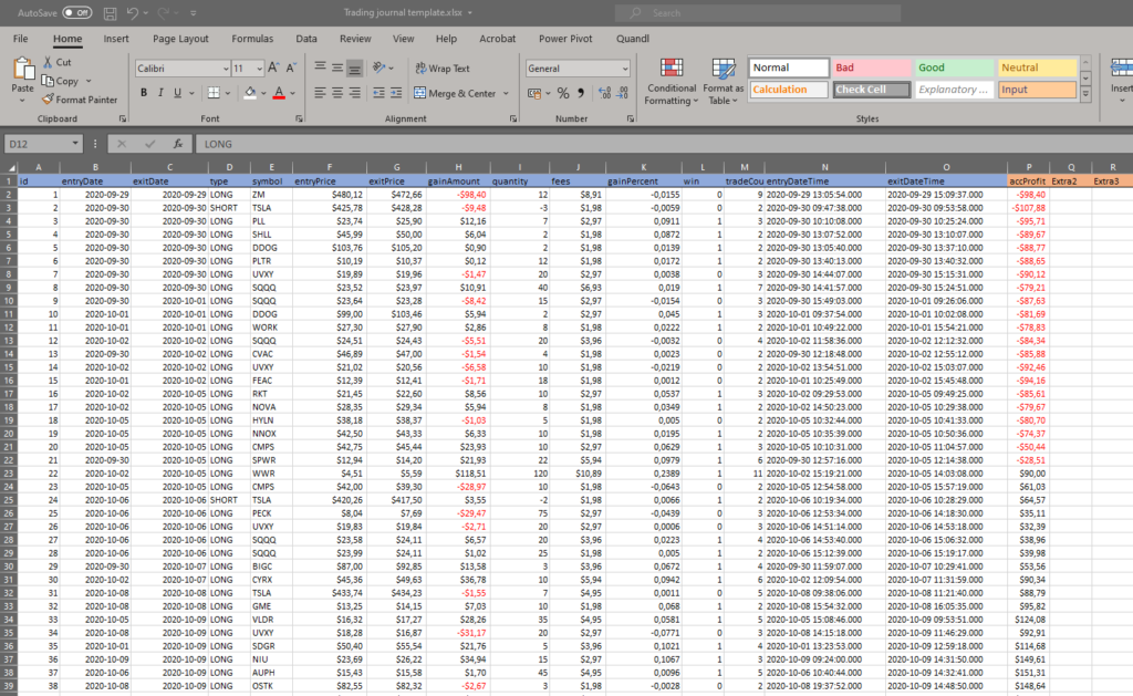
Column P in the example above is a calculated column to get accumulated profit.
You can compute the accumulated profit by summarizing the gainAmount column and the previous row and repeat until the end.
When you have added some data you need to add a named range.
- Select All columns containing data and all cells down to some number you will never reach
- Open the formulas menu and select Define name
- Define a new name and name it trades
Adding pivot tables
Create anew sheet and name it pivots.
We are going to create 8 pivot tables, one for each chart or value we want to display on the dashboard.
After you are done you should have a sheet looking like this
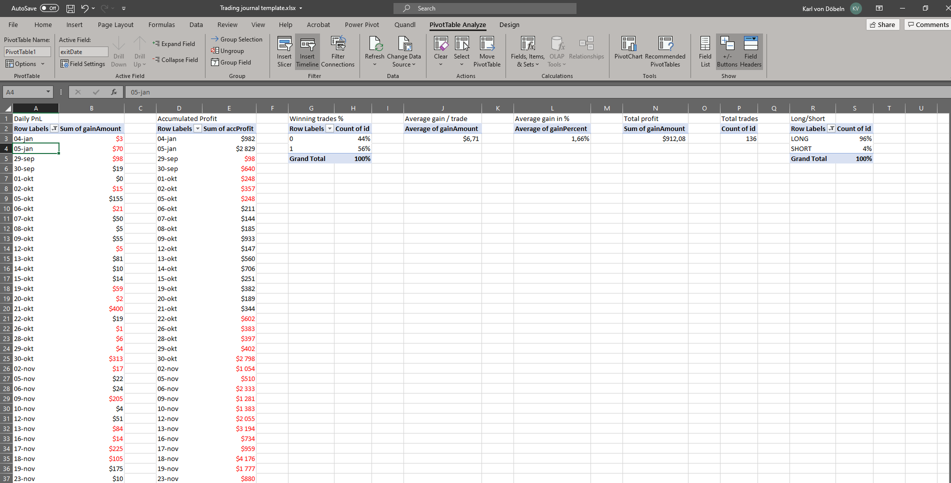
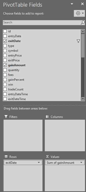
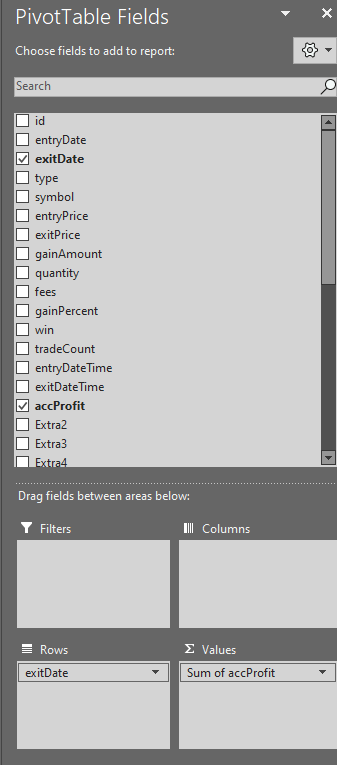
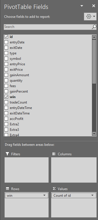
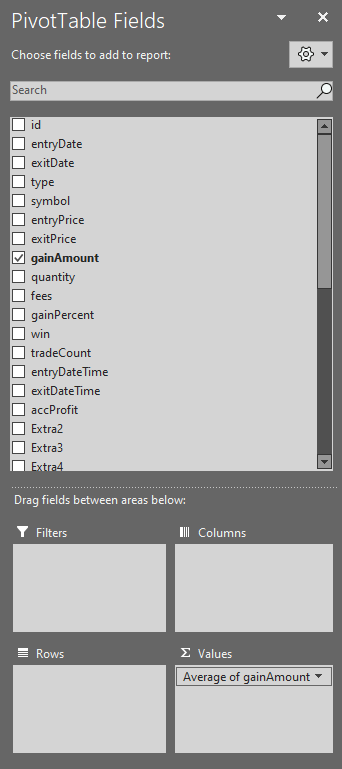
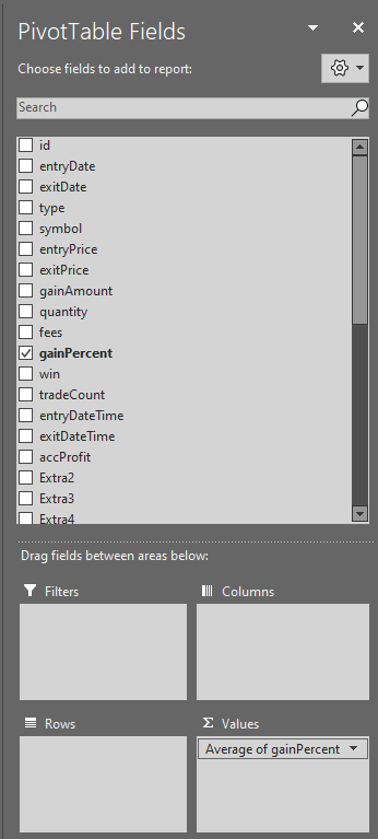
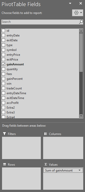
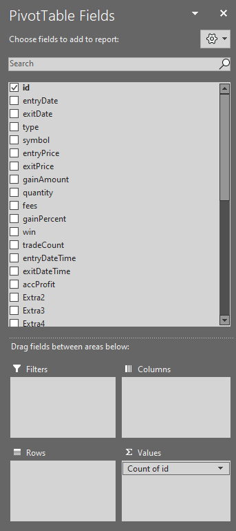
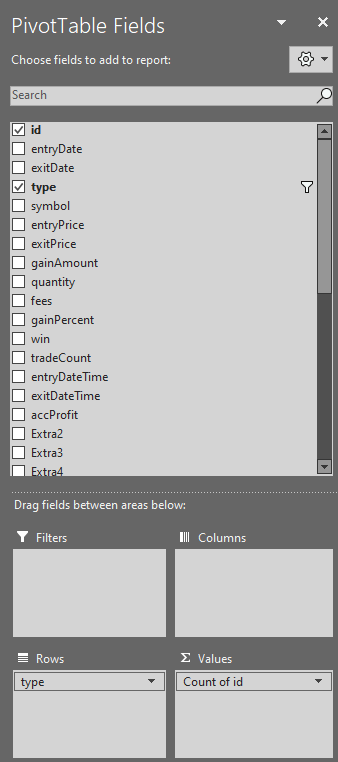
Below is the configuration used for each Pivot added
Pivot 1, Daily PnL
Pivot 2, Winning trades %
Pivot 3, Average gain / trade
Pivot 4, Average gain in %
Pivot 5, Average gain in %
Pivot 6, Total profit
Pivot 7, Total trades
Pivot 8, Long/short
Adding slicers
Select any of the pivot tables to show the field list.
- Right-click on Months and select Add as slicer
- Right-click on Years and select Add as slicer
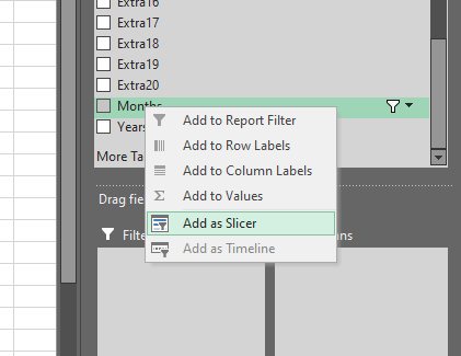
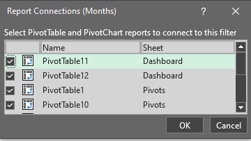
Right-click on the newly added Month slicer and select Report connections.
Check all the checkboxes for the other pivot tables
Repeat for the Years slicer
Creating the Charts
With a pivot table selected you get a menu choice, PivotTable Analyze
- Open the PivotTable Analyze menu
- Select PivotChart under the Tools section
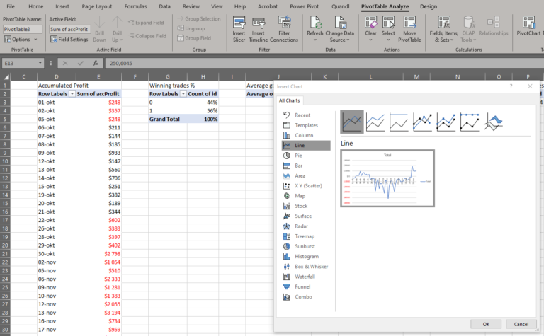
In the example above we add a Line Chart for the accumulated profit but you could of course select a different Chart type and styling
Add a chart using the same method for Daily PnL, for example a Line Chart or a Bar Chart
Add a chart using the same method for Long/Short, for example a Pie Chart
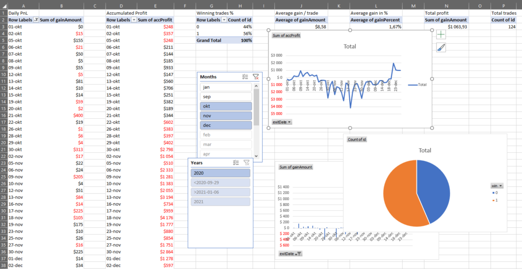
When done you should have 2 slicers and a few charts in the Pivots sheet.
Creating the Dashboard
Now that you have the charts and slicers we are going to create the dahsboard.
Add a new sheet and name it Dashboard
From the Pivots sheet, select the slicers and the charts (only these and not any data from the sheet), cut them out (Ctrl-X).
Switch to your Dashboard sheet and paste them.
Decide on 4 fields which are going to be used for data about
- Total PnL
- Wins
- Avg gain / trade
- Avg gain / trade %
- Total trades
- Select the cell
- press =
- Switch to the Pivot table sheet
- Select the appropriate value cell in the Pivot table
- Press Enter

Repeat the above for the other values you want to display on your dashboard.
Adjust the format of the values depending on what the value represents, winning trades should be displayed as a % and Total profit as currency.
Finally, adjust font-sizes, size of the charts, move things around, and add some colors to make it look nice.
I like to have Slicers on top on one row to make as much room as possible for the charts.
When you are done, it may look something like this.
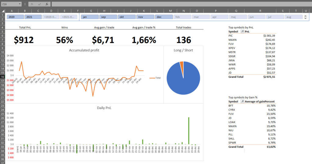
Since the slicers are linked to all pivot tables and charts are based on those pivot tables, you can update the time-frame for the whole dashboard using the slicers.
Download
Tutorials are great but sometimes you just want to Download a pre-made Trading Journal Template in Excel.
Learn more
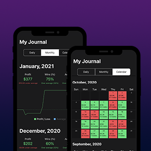
The kinfo Social Trading Journal
Learn more about how you can utilize kinfo as an automated trading journal
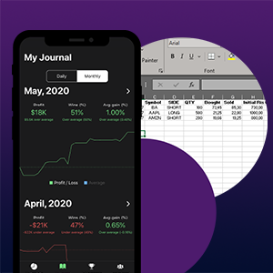
What is a Trading Journal
Learn more about how you can utilize kinfo as an automated trading journal
